A Surprising Pitfall of Human Judgement and How to Correct It

Introduction

Algorithms based on machine learning, deep learning, and AI are in the news these days. Evaluating the quality of these algorithms is usually done using human judgment. For example, if an algorithm claims to detect whether an image contains a pet, the claim can be checked by selecting a sample of images, using human judges to detect if there is a pet, and then comparing this to the results to the algorithm. This post discusses a pitfall in using human judgment that has been mostly overlooked until now.

In real life, human judges are imperfect. This is especially true if the judges are crowdsourced. This is not a new observation. Many proposals to process raw judgment scores and improve their accuracy have been made. They almost always involve having multiple judges score each item and combining the scores in some fashion. The simplest (and probably most common) method of combination is majority vote: for example, if the judges are rating yes/no (for example, is there a pet), you could report the rating given by the majority of the judges.

But even after such processing, some errors will remain. Judge errors are often correlated, and so multiple judgments can correct fewer errors than you might expect. For example, most of the judges might be unclear on the meaning of “pet”, incorrectly assume that a chicken cannot be a pet, and wrongly label a photo of a suburban home showing a child playing with chickens in the backyard. Nonetheless, any judgment errors remaining after processing are usually ignored, and the processed judgments are treated as if they were perfect.

Ignoring judge errors is a pitfall. Here is a simulation illustrating this. I’ll use the pet example again. Suppose there are 1000 images sent to the judges and that 70% of the images contain a pet. Suppose that when there is no pet, the judges (or the final processed judgment) correctly detect this 95% of the time. This is actually higher than typical for realistic industrial applications. And suppose that some of the pet images are subtle, and so when there is a pet, judges are correct only 90% of the time. I now present a simulation to show what happens.

Here’s how one round of the simulation works. I assume that there are millions of possible images and that 70% of them contain a pet. I draw a random sample of 1000. I assume that when the image has a pet, the judgment process has a 90% chance reporting “pet”, and when there is no pet, the judgment process reports “no pet” 95% of the time. I get 1000 judgments (one for each image), and I record the fraction of those judgments that were “pet”.

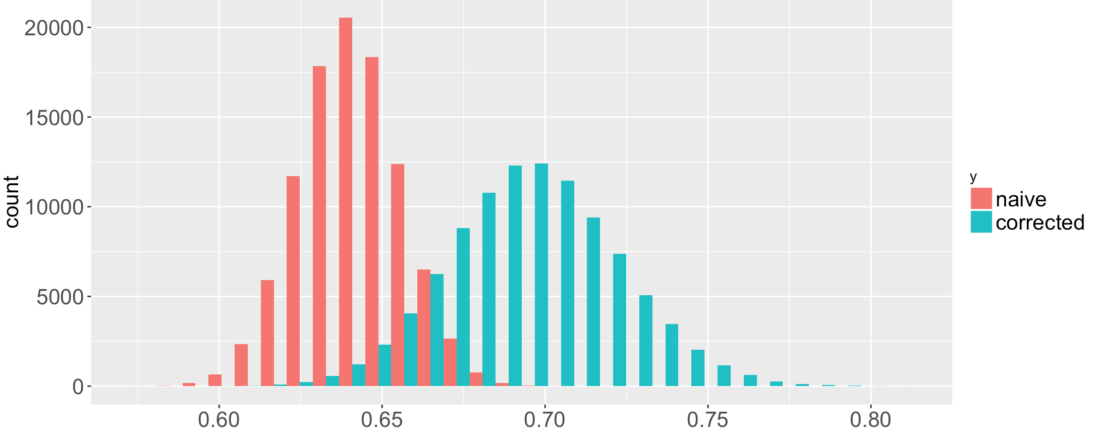
That’s one round of the simulation. I do the simulation many times and plot the results as a histogram. I actually did 100,000 simulations, so the histogram has 100,000 values. The results are below in red. Since this is a simulation, I know the true fraction of images with pets: it’s 70%. The estimated fraction from the judges in each simulation is almost always lower than the true fraction. Averaged over all simulations, the estimated fraction is 64%, noticeably lower than the true value of 70%.

This illustrates the pitfall: by ignoring judge error, you get the wrong answer. You might wonder if this has any practical implications. How often do you need a precise estimate for the fraction of pets in a collection of images? But what if you’re using the judgments to determine the accuracy of an algorithm that detects pets? And suppose the algorithm has an accuracy rate of 70%, but the judges say it is 64%. In the machine learning/AI community, the difference between an algorithm that is 70% accurate vs 64% is a big deal.

But maybe things aren’t as bad as they seem. When statistically savvy experimenters report the results of human judgment, they return error bars. The error bars (I give details below) in this case are

   

So even error bars don’t help: the actual accuracy rate of 0.7 is not included inside the error bars.

The purpose of this post is to show that you can compensate for judge error. In the image above, the blue bars are the simulation of the compensating algorithm I will present. The blue bars do a much better job of estimating the fraction of pets than the naive algorithm. This post is just a summary, but full details are in Drawing Sound Conclusions from Noisy Judgments from the WWW17 conference.

The histogram shows that the traditional naive algorithm (red) has a strong bias. But it also seems to have a smaller variance, so you might wonder if it has a smaller mean square error (MSE) than the blue algorithm. It does not. The naive algorithm has MSE 0.0037, the improved algorithm 0.0007. The smaller variance does not compensate for the large bias.

Finally, I can explain why judge error is so important. For a typical problem requiring ML/AI, many different algorithms are tried. Then human judgment can be used to detect if one is better than the other. Current practice is to use error bars as above, which do not take into account errors in the human judgment process. But this can lead the algorithm developer astray and suggest that a new algorithm is better (or worse) when in fact the difference is just noise.

The setup

I’m going to assume there are both an algorithm that takes an input and outputs a label (not necessarily a binary label) and also a judge that decides if the output is correct. So the judge is performing a binary task: determining if the algorithm is correct or not. From these judgments, you can compute the fraction of times (an estimate of the probability ) that the algorithm is correct. I will show that if you can estimate the error in the judgment process, then you can compensate for it and get a better estimate of the accuracy of the algorithm. This applies if you use raw judge scores or if you use a judgment process (for example, majority vote) to improve judge accuracy. In the latter case, you need to estimate the accuracy of the judgment process.

A simple example of this setup is an information retrieval algorithm. The algorithm is given a query and returns a document. A judge decides if the document is relevant or not. A subset of those judgments is reevaluated by gold judge experts, giving an estimate of the judges’ accuracy. Of course, if you are rich enough to be able to afford gold judges to perform all your labeling, then you don’t need to use the method presented here.

A slightly more subtle example is the pet detection algorithm mentioned above. Here it is likely that there would be a labeled set of images (a test set) used to evaluate the algorithm. You want to know how often the algorithm agrees with the labels, and you need to correct for errors in the judgment about agreement. To estimate the error rate, pick a subset of images and have them rejudged by experts (gold judges). The judges were detecting if an image had a pet or not. However, what I am really interested in is the error rate in judging whether the algorithm gave the correct answer or not. But that is easily computed from the gold judgments of the images.

The first formula

In the introduction, I mentioned that there are formulas that can correct for judge error. To explain the formula, recall that there is a task that requires labeling items into two classes, which I’ll call positive and negative. In the motivating example, positive means the algorithm gives the correct output for the item, negative that it is incorrect. I have a set of items, and judges perform the task on each item, getting an estimate of how many items are in the positive class. I’d like to use information on the accuracy of the judges to adjust this estimate. The symbols used in the formula are:

The first formula is

   

This formula is not difficult to derive. See the aforementioned WWW paper for details. Here are some checks that the formula is plausible. If the judges are prefect then , and the formula reduces to . In other words, the judges’ opinion of is correct. Next, suppose the judges are useless and guess randomly. Then , and the formula makes no sense because the denominator is infinity. So that’s also consistent.

Notice the formula is asymmetric: the numerator has but not . To see why this makes sense, first consider the case when the judges are perfect on negative items so that . The judges’ only error is to take correct answers and claim they are negative. So an estimate of by the judges is always too pessimistic. On the other hand, if , then the judges are optimistic, because they sometimes judge incorrect items as correct.

I will now show that the formula achieves these requirements. In particular, if then I expect and if then . To verify this, note that if the formula becomes . And if then

   

the last inequality because and .

Up until now the formula is theoretical, because the precise values of , and are not known. I introduce some symbols for the estimates.

The practical formula is

   

The second formula

In the introduction, I motivated the concern with judgment error using the problem of determining the accuracy of an ML algorithm and, in particular, comparing two algorithms to determine which is better. If you had perfect judges and an extremely large set of labeled data, you could measure the accuracy of each algorithm on the large labeled set, and the one with the highest accuracy would clearly be best. But the labeled set is often limited in size. That leads to some uncertainty: if you had picked a different labeled set you might get a difference answer. That is the purpose of error bars: they quantify the uncertainty. Traditionally, the only uncertainty taken into account is due to the finite sample size. In this case, the traditional method gives 95% error bars of where

   

The judge gave a positive label times out of , is the estimated mean and the estimate of the variance of . I showed via simulation that if there are judgment errors, these intervals are too small. The corrected formula is

   

where

The formula shows that when taking judge error into account, the variance increases, that is, . The first term of the equation for is already larger than , since is it divided by a number less than one. The next two terms add additional error, due to the uncertainty in estimating the judge errors and .

Extensions

The theme of this post is correcting for judge errors, but I have only discussed the case when the judge gives each item a binary rating, as a way to estimate what fraction of items are in each of the two classes. For example, the judge reports if an algorithm has given the correct answer, and you want to know how often the algorithm is correct. Or the judge examines a query and a document, and you want to know how often the document is relevant to the query.

But the methods presented so far extend to other situations. The WWW paper referred to earlier gives a number of examples in the domain of document retrieval. It explains how to correct for judge error in the case when a judge gives documents a relevance rating rather than just a binary relevant or not. And it shows how to extend these ideas beyond the metric “fraction in each class” to the metric DCG, which is a common metric for document retrieval.

Assumptions

Analyses of the type presented here always have assumptions. The assumption of this work is that there is a task (for example, “is the algorithm correct on this item?”) with a correct answer and that there are gold judges who are expert enough and have enough time to reliably obtain that correct answer. Industrial uses of human judgment often use detailed guidelines explaining how the judgment should be done, in which case these assumptions are reasonable.

But what about the general case? What if different audiences have different ideas about the task? For example, there may differences from country to country about what constitutes a pet. The analysis presented here is still relevant. You only need to compute the error rate of the judges relative to the appropriate audience.

I treat the judgment process as a black box, where only the overall accuracy of the judgments is known. This is sometimes very realistic, for example, when the judgment process is outsourced. But sometimes details are known about the judgment process would lead you to conclude that the judgments of some items are more reliable than others. For example, you might know which judges judged which items, and so have reliable information on the relative accuracy of the judges. The approach I use here can be extended to apply in these cases.

The simulation

I close this post with the R code that was used to generate the simulation given earlier.

# sim() returns a (n.iter x 4) array, where each row contains:
#   the naive estimate for p,
#   the corrected estimate,
#   whether the true value of p is in a 95% confidence interval (0/1)
#        for the naive standard error
#   the same value for the corrected standard error

sim = function(
  q.pos,  # probability a judge is correct on positive items
  q.neg,  # probability a judge is correct on negative items
  p,      # fraction of positive items
  n,      # number of items judged
  n.sim,  # number of simulations
  n.gold.neg = 200, # number of items the gold judge deems negative
  n.gold.pos = 200  # number of items the gold judge deems positive
  )
{
   # number of positive items in sample
   n.pos = rbinom(n.sim, n, p)

   # estimate of judge accuracy
   q.pos.hat = rbinom(n.sim, n.gold.pos, q.pos)/n.gold.pos
   q.neg.hat = rbinom(n.sim, n.gold.neg, q.neg)/n.gold.neg

   # what the judges say (.jdg)
   n.pos.jdg = rbinom(n.sim, n.pos, q.pos) +
               rbinom(1, n - n.pos, 1 - q.neg)

   # estimate of fraction of positive items
   p.jdg.hat = n.pos.jdg/n    # naive formula
   # corrected formula
   p.hat = (p.jdg.hat - 1 + q.neg.hat)/
                      (q.neg.hat + q.pos.hat - 1)

   # is p.jdg.hat within 1.96*sigma of p?
   s.hat =  sqrt(p.jdg.hat*(1 - p.jdg.hat)/n)
   b.jdg = abs(p.jdg.hat - p) < 1.96*s.hat

   # is p.hat within 1.96*sigma.hat of p ?
   v.b = q.neg.hat*(1 - q.neg.hat)/n.gold.neg   # variance q.neg
   v.g = q.pos.hat*(1 - q.pos.hat)/n.gold.pos
   denom = (q.neg.hat + q.pos.hat - 1)^2
   v.cor = s.hat^2/denom +
           v.g*(p.jdg.hat - 1 + q.neg.hat)^2/denom^2 +
           v.b*(p.jdg.hat - q.pos)^2/denom^2
   s.cor.hat = sqrt(v.cor)
   # is negative.jdg.rate.cor within 1.96*sigma of p?
   b.cor = abs(p.hat - p) < 1.96*s.cor.hat

   rbind(p.jdg.hat, p.hat, b.jdg, b.cor)
}

set.seed(13)
r = sim(n.sim = 100000, q.pos = 0.90,  q.neg = 0.95, p = 0.7, n=1000)

# plot v1 and v2 as two separate histograms, but on the same ggplot
hist2 = function(v1, v2, name1, name2, labelsz=12)
{
  df1 = data.frame(x = v1, y = rep(name1, length(v1)))
  df2 = data.frame(x = v2, y = rep(name2, length(v2)))
  df = rbind(df1, df2)

  freq = aes(y = ..count..)
  print(ggplot(df, aes(x=x, fill=y)) + geom_histogram(freq, position='dodge') +
      theme(axis.text.x = element_text(size=labelsz),
      axis.text.y = element_text(size=labelsz),
      axis.title.x = element_text(size=labelsz),
      axis.title.y = element_text(size=labelsz),
      legend.text = element_text(size=labelsz))
  )
}

hist2(r[1,], r[2,], "naive", "corrected", labelsz=16)

---

Powered by QuickLaTeX.