In the first part of this blog posting, I talked about how to estimate a buyer’s propensity to purchase an auction over a fixed price item. I gave the Empirical Bayes formula f = (a+k)/(a + b+ n) for the auction propensity f which is a compromise between the buyer’s shopping history k/n and the propensity of his peer group a/(a+b). In this posting I will explain where the formula comes from, and how to compute the numbers a and b.
Since the method is called Empirical Bayes, it won’t surprise you to learn that it uses Bayes Theorem
![]()
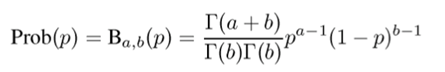
The specific form I’ll use is
![]()
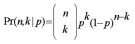
In this formula, p is the probability of buying an auction, n is the number of purchases that a shopper has made, and k is the number of those purchases that were auctions. The left-hand side is what I’d like to know: the probability (propensity) of an auction given that the buyer has previously purchased k/n auctions. As usual, the reason to use Bayes formula is that it relates the unknown left-hand side to the computable right-hand side.
The pleasure of Bayes formula is the first term on the right-hand side. This is the textbook formula we’ve seen before:
The pain of Bayes formula is the second term, the prior Pr(p). This is the estimate of p before (prior to) learning there were k/n auction purchases. Much time has been spent debating what value to use for the prior. This is where empirical Bayes comes in. I will use the data itself to estimate Pr(p). I do it by assuming that Pr(p) follows a Beta probability distribution
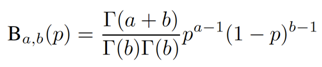
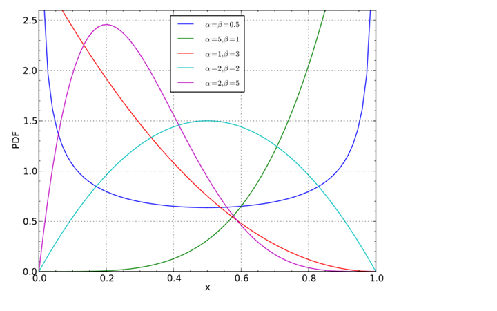
and all I need to do is specify the two parameters a and b. Why this distribution? It’s general enough to fit most data, but simple enough to make explicit calculations possible. I’ll do those calculations in a moment. The following figure from Wikipedia shows the first point. By varying the parameters a and b (α and β in the figure) you can get a large range of distributions.
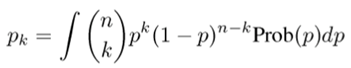
Now for the details of how to compute a and b. The probability of purchasing k/n auctions is
![]()
If I don’t know a precise value for p, but do know it varies via some probability distribution Prob(p) then pk is an average over those p, expressed as the integral
As I mentioned above, I’ll assume that Prob(p) is a beta distribution
Now plug this value of Prob(p) into the formula for pk which I’ve written as pk(a, b) to emphasize the dependence on a and b.
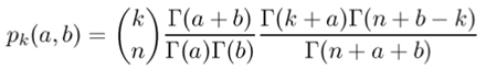
If you’re following along in detail, you’ll see that I did some simplifications after the plug-in. The important thing is this: the value of pk depends on the known k, n and the unknown a, b, and my job is to pick those a, b so that
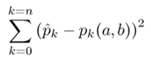
is minimized. In other words, I want to make the computed pk as close as possible to the observed fraction, which I’ve written with a hat. For example p2 (a,b) is the computed fraction of people in the peer group that bought 2 auctions assuming the prior is Beta(a, b), while p2 with a hat is the observed fraction of users who bought two auctions.
Here’s an illustration. Suppose the peer group is users who’ve purchased 21 items. Then the best values of a and b are 1.16 and 2.22 which gives this beta distribution:

Once I have a and b I can compute the pk (a,b) and see how closely they approximate

The match is excellent. The red predicted curve has only two parameters and yet it has a very good fit to all 22 points.
Now that I’ve explained how to compute a and b, I can explain where the formula f = (a+k)/(a + b+ n) comes from. Use Bayes formula
![]()
and substitute the beta distribution Ba,b for Pr(p) as follows:

I’ve been a little pedantic and used â to show that it is an estimate of a derived from the peer group (and similarly for b). The calculations above show that when you plug the formula for Ba,b(p) into Bayes formula you get out another beta distribution! This is the explanation for my earlier statement that beta was chosen to make explicit calculations possible.
My goal is to estimate the auction propensity for a buyer who has purchased k/n auctions. What I have so far is a probability distribution for this propensity, specifically a beta distribution. If I want a single probability, the natural choice is the average of that beta distribution. The average of Beta(a,b) is a/(a+b). So if I want to get a single number for the auction propensity, I take the average of
![]()
which is (a+k)/(a+b+n). This is the formula that I have used many times in this posting.
So much for the calculations. I want to end by discussing whether personalization is desirable. Some have argued that it isn’t a good idea to show users only what they’ve seen before. I think these arguments are often attacking a straw man. A good personalization system doesn’t eliminate all variety, it merely tailors it. Suppose our Mr. X has purchased 20 items, all of them at fixed price. But his friend Ms. Y has done the opposite: all her purchases were made by auction. I find it hard to believe that anyone would seriously argue that X and Y should see the same search results. Just as bad as showing X a pile of auctions would be to never show him any auctions. A good personalization system should be nuanced. Methods like those shown in this posting provide principled estimates of user’s preferences. But how these preferences are used requires some finesse.