A Case Study in Empirical Bayes

Empirical Bayes is a statistical technique that is both powerful and easy to use. My goal is to illustrate that statement via a case study using eBay data. Quoting the famous statistician Brad Efron,

Empirical Bayes seems like the wave of the future to me, but it seemed that way 25 years ago and the wave still hasn’t washed in, despite the fact that it is an area of enormous potential importance.

Hopefully this post will be one small step in helping Empirical Bayes to wash in! The case study I’ll present comes from ranking the items that result from a search query. One feature that is useful for ranking items is their historical popularity. On eBay, some items are available in multiple quantities. For these, popularity can be measured by the number of times an item is sold divided by the number of times it is displayed, which I will call sales/impressions (S/I). By the way, everything I say applies to any ratio of counts, not just sales and impressions.

The problem

The problem I want to discuss is what to do if the denominator is small. Suppose that items typically have 1 sale per 100 impressions. Now suppose that a particular item gets a sale just after being listed. This is a typical item that has a long-term S/I of about 0.01, but by chance it got its sale early, say after the 3rd impression. So S/I is 1/3, which is huge. It looks like an enormously popular item, until you realize that the denominator I is small: it has received only 3 impressions. One solution is to pass the problem downstream, and give the ranker both S/I and I. Let the ranker figure out how much to discount S/I when I is small. Passing the buck might make sense in some situations, but I will show that it’s not necessary, and that it’s possible to pass a meaningful value even when I is small.

How to do that? Informally, I want a default value of S/I, and I want to gradually move from that default to the actual S/I as I increases. Your first reaction is probably to do this by picking a number (say 100), and if I < 100 use the default, otherwise S/I. But once you start to wonder whether 100 is the right number, you might as well go all the way and do things in a principled way using probabilities.

The solution

Jumping to the bottom line: the formula will be (S + α)/(I + γ). This clearly satisfies the desire to be near S/I when S and I are large. It also implies that the default value is α/γ, since that’s what you get when S=I=0. In the rest of this post I will explain two things. First, how to pick α and γ (there is a right way and a wrong way). And second, where the shape of the formula (S + α)/(I +γ) comes from. If you’re familiar with Laplace smoothing then you might think of using (S+1)/(I+1), and our formula is a generalization of that. But it still begs the question — why a formula of this form, rather than, for example, a weighted sum $(1 - e^{-\alpha I})(S/I) + e^{-\alpha I}(\alpha/\gamma)$ .

The formula (S + α)/(I +γ) comes by imagining that at each impression, there is a probability of an associated sale, and then returning the best estimate of that probability instead of returning S/I. I’ll start with the simplest way of implementing this idea (although it is too simple to work well).

Suppose the probability of a sale has a fixed universal value , so that whenever a user is shown an item, there is a probability that the item is sold. This is a hypothetical model of how users behave, and it’s straightforward to test if it fits the data. Simply pick a set of items, each with an observed sale count and impression count. If the simple model is correct, then an item with impressions will receive sales according to the binomial formula:

$\Pr(\mbox{getting } k \mbox{ sales}) = \binom{n}{k} p^{k}(1-p)^{n - k}$

Here is the number of impressions and the number of sales. As mentioned earlier, this whole discussion also works for other meanings of and , such as is clicks and is impressions. To test the simple model, I can compare two sets of data. The first is the observed pairs . In other words, I retrieve historical info for each item, and record impressions and sales. I construct the second set by following the simple model: I take the actual number of impressions , and randomly generate the number of sales according to the formula above. Below is a histogram of the two data sets. Red is simulated (the model), and blue is actual. The match is terrible.

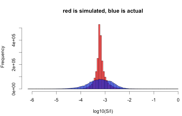
Here is some more detail on the plot: Only items with a nonzero sale count are shown. In the simulation there are 21% items with S=0, but the actual data has 47%.

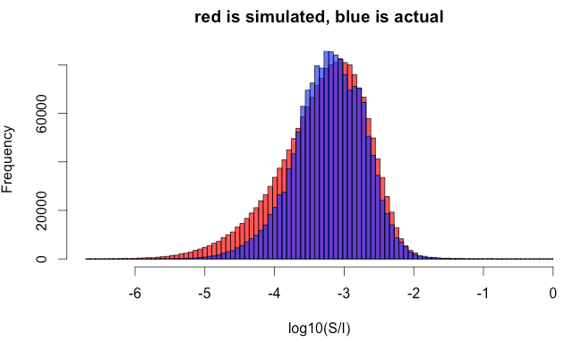
So we need to go to a more sophisticated model. Instead of a fixed value of , imagine drawing from a probability distribution and plugging it into the inset equation, which is then used to get the random . As you can see in the plot below, the two histograms have a much more similar shape than the previous plot, and so this model does a better job of matching the actual data.

Now it all boils down to finding the distribution for . Since $0 \leq p \leq 1$ , that means finding a probability distribution on the interval [0, 1]. The most common such distribution is the Beta distribution, which has two parameters, $\alpha$ and $\beta$ . By assuming a Beta distribution, I reduce the problem to finding $\alpha$ and $\beta$ (and yes, this α is the same one as in the formula (S + α)/(I +γ)). This I will do by finding the values of $\alpha$ and $\beta$ that best explain the observed values of and . Being more precise, associated to each of historical items is a sale count and an impression count , with $1 \leq i \leq N$ .

I was perhaps a bit flip in suggesting the Beta distribution because it is commonly used. The real reason for selecting Beta is that it makes the computations presented in the Details section below much simpler. In the language of Bayesian statistics, the Beta distribution is conjugate to the binomial.

At this point you can fall into a very tempting trap. Each is a number between 0 and 1, so all the values form a histogram on [0,1]. The possible values of follow the density function for the Beta distribution and so also form a histogram on [0,1]. Thus you might think you could simply pick the values of $\alpha$ and $\beta$ that make the two histograms match as closely as possible. This is wrong, wrong, wrong. The values are from a discrete distribution and often take on the value 0. The values of come from a continuous distribution (Beta) and are never 0, or more precisely, the probability that is 0. The distributions of and of are incompatible.

In my model, I’m given and I spit out by drawing from a Beta distribution. The Beta is invisible (latent) and indirectly defines the model. I’ll give a name to the output of the model: . Restating, fix an and make a random variable that produces value with the probability controlled indirectly by the Beta distribution. I need to match the observed (empirical) values of to X, not to Beta. This is the empirical Bayes part. I’ll give an algorithm that computes $\alpha$ and $\beta$ later.

But first let me close the loop, and explain how all this relates to (S + α)/(I + γ). Instead of reporting S/I, I will report the probability of a sale. Think of the probability as a random variable — call it . I will report the mean value of the random variable . How to compute that? I heard a story about a math department that was at the top of a tall building whose windows faced the concrete wall of an adjacent structure. Someone had spray-painted on the wall “don’t jump, integrate by parts.” If it had been a statistics department, it might have said “don’t jump, use Baye’s rule.”

Baye’s rule implies a conditional probability. I want not the expected value of , but the expected value of conditional on impressions and sales. I can compute that from the conditional distribution $\Pr(P = p \:|\: (n,k))$ . To compute this, flip the two sides of the | to get $\Pr((n,k) \:|\: P=p)$ . This is $\Pr(\mbox{getting } k \mbox{ sales})$ , which is just the inset equation at the beginning of this post!

Now you probably know that in Baye’s rule you can’t just flip the two sides, you also have to include the prior. The formula is really $\Pr(P = p \:|\: (n,k)) = \mbox{constant} \times \Pr((n,k) \:|\: P = p) \Pr(P=p)$ . And $\Pr (P=p)$ is what we decided to model using the Beta distribution with parameters $\alpha$ and $\beta$ . These are all the ingredients for Empirical Bayes. I need $\Pr(P = p \:|\: (n,k))$ , I evaluate it using Baye’s rule, the rule requires a prior, and I use empirical data to pick the prior. In empirical Bayes, I select the prior that best explains the empirical data. For us, the empirical data is the observed values of . When you do the calculations (below) using the Beta $(\alpha, \beta)$ distribution as the prior, you get that the mean of P is (S + α)/(I + γ) where γ = α + β.

How does this compare with the simplistic method of using S/I when I > δ, and η otherwise? The simplistic formula involves two constants δ and η just as the principled formula involves two constants α and γ. But the principled method comes with an algorithm for computing α and γ given below. The algorithm is a few lines of R code (using the optimx package).

The details

I’ll close by filling in the details. First I’ll explain how to compute $\alpha$ and $\beta$ .

I have empirical data on items. Associated with the -th item ( $1 \leq i \leq N$ ) is a pair , where might be the number of sales and the number of impressions, but the same reasoning works for clicks instead of sales. A model for generating the is that for each impression there is a probability that the impression results in a sale. So given , the probability that is $\binom{n_i}{j} p^{j}(1-p)^{n_i - j}$ . Then I add in that the probability is itself random, drawn from a parametrized prior distribution with density function $f_\theta(p)$ . I generate the in a series of independent steps. At step , I draw from $f_\theta(p)$ , and then generate according to the binomial probability distribution on :

$\mbox{Prob}(k_i = j) = \binom{n_i}{j} p_i^{j}(1-p_i)^{n_i - j}$

Using this model, the probability of seeing given is computed by averaging over the different possible values of , giving

$q_i(\theta) = \int_0^1 \binom{n_i}{k_i} p^{k_i}(1-p)^{n_i - k_i} f_\theta(p) dp$

I’d like to find the parameter $\theta$ that best explains the observed and I can do that by maximizing the probability of seeing all those . The probability seeing is $q_i(\theta)$ , the probability of seeing the whole set is $\prod_i q_i(\theta)$ and the log of that probability is $\sum_i \log q_i(\theta)$ . This is a function of $\theta$ , and I want to find the value of $\theta$ that maximizes it. This log probability is conventionally called the log-likelihood.

Since I’m assuming $f_\theta(p)$ is a beta distribution, with $\theta = (\alpha, \beta)$ , then $q_i(\theta)$ becomes

$\begin{eqnarray*} q_i(\alpha, \beta) & = & \binom{n_i}{k_i} \int_0^1 p^{k_i}(1-p)^{n_i - k_i} \frac{ \Gamma(\alpha + \beta)}{\Gamma(\alpha)\Gamma(\beta)} p^{\alpha-1}(1-p)^{\beta-1} dp \\ & = & \binom{n_i}{k_i} \frac{ \Gamma(\alpha + \beta)}{\Gamma(\alpha)\Gamma(\beta)} \int_0^1 p^{k_i + \alpha -1}(1-p)^{n_i +\beta - k_i - 1} dp \\ & = & \binom{n_i}{k_i} \frac{B(\alpha + k_i, n_i + \beta - k_i)}{B(\alpha, \beta)} \end{eqnarray*}$

The calculation above uses the definition of the beta function and the formula for the beta integral

$\begin{eqnarray*} B(\alpha,\beta) & = & \frac{\Gamma(\alpha)\Gamma(\beta)}{\Gamma(\alpha+\beta)} \\ \int_0^1 x^{\alpha-1} (1-x)^{\beta-1} dx & = & B(\alpha, \beta) \end{eqnarray*}$

If you don’t want to check my calculations, $q_i(\alpha, \beta)$ is just the beta-binomial distribution, and you can find its formula in many books and web pages.

Restating, to find $\alpha$ , $\beta$ is to maximize the log-likelihood $l(\alpha, \beta) = \sum_i \log q_i(\alpha, \beta)$ , specifically

$l(\alpha, \beta) = \sum_i \left( \log \binom{n_i}{k_i} + \log B(\alpha + k_i, n_i + \beta - k_i) - \log B(\alpha, \beta) \right)$

And since the first term doesn’t involve $\alpha$ or $\beta$ , you only need to maximize

$\sum_{i=1}^N \log B(\alpha + k_i, n_i + \beta - k_i) - N\log B(\alpha, \beta)$

The method I used to maximize that expression was the optimx package in R.

The final missing piece is why, when I replace S/I with the probability that an impression leads to a sale, the formula is $(k + \alpha)/(n + \gamma)$ .

I have an item with an unknown probability of sale . All that I do know is that it got sales out of impressions. If is the random variable representing the sale probability of an item, and is a random variable representing the sale/impression of an item, I want $\Pr(P = p \:|\: F = (k, n))$ , which I write as $\Pr(p \:|\: k, n)$ for short. Evaluate this using Baye’s rule,

$\Pr(p \:|\: k, n) = \Pr(k,n \:|\: p) \Pr(p) / \Pr(k,n)$

The $\Pr(k,n)$ term can be ignored. This is not deep, but can be confusing. In fact, any factor $\phi(k,n)$ involving only and (like $1/\Pr(k,n)$ ) can be ignored. That’s because $\int \Pr(p \:|\: k, n) dp = 1,$ so if $\Pr(p \:|\: k, n) =f(p,k,n)\phi(k,n)$ it follows that $\phi$ can be recovered from using $\phi(k,n) = 1/\int(f(p,k,n)dp.$ In other words, I can simply ignore a $\phi$ and reconstruct it at the very end by making sure that $\int \Pr(p \:|\: k, n) dp = 1$ .

I know that

$\Pr(k,n \:|\: p) = \binom{n}{k} p^k(1-p)^{n-k}$

For us, the prior $\Pr(p) = f_\theta(p) = f_{\alpha, \beta}(p)$ is a beta distribution, $\mbox{Beta}_{\alpha, \beta}(p) =$ $p^{\alpha-1}(1~-~p)^{\beta-1}/B(\alpha, \beta)$ . Some algebra then gives

$\\Pr(p \:|\: k, n) \propto \Pr(k,n \:|\: p) \Pr(p) \propto \mbox{Beta}_{\alpha + k, \beta + n - k}(p)$

The $\propto$ symbol ignores constants involving only and . Since the rightmost term integrates to 1, the proportionality is an equality:

$\Pr(p \:|\: k, n) = \mbox{Beta}_{\alpha + k, \beta + n - k}(p)$

For an item with I want to know the value of , but this formula gives the probability density for . To get a single value I take the mean, using the fact that the mean of $\mbox{Beta}_{\alpha, \beta}$ is $\alpha/(\alpha+\beta)$ . So the estimate for is

$\mbox{Mean}(\mbox{Beta}_{\alpha + k, \beta + n - k}) = \frac{\alpha + k}{\alpha + \beta + n}$

This is just (S + α)/(I + γ) with γ = α + β.

There’s room for significant improvement. For each item on eBay, you have extra information like the price. The price has a big effect on S/I, and so you might account for that by dividing items into a small number of groups (perhaps low-price, medium-price and high-price), and computing $\alpha$ , $\beta$ for each. There’s a better way, which I will discuss in a future post.

Tags: Applied Math, Search Science