Portico

About three years ago, the Decide.com team joined eBay, and we started working on eBay Insights with a mission to bring powerful analytics to eBay sellers. Later, seller analytics became a key component of Seller Hub. Seller Hub is eBay’s one-stop portal, providing a unified platform for millions of eBay professional sellers. It is the hub where sellers get access to all the summaries, activities, tools, and insights about their businesses on eBay.

Seller analytics in Seller Hub is powered by Portico — a data store that we built in house to support interactive, sub-second, complex aggregations on top of hundreds of billions of listing, purchase, behavioral activity tracking, and other kinds of records, with dozens of trillions of data elements, covering several years of listing history. Portico is currently handling millions of queries daily providing market GMV, traffic report, competitor analysis, and recommendations for unlikely to sell items through Performance and Growth tabs in Seller Hub.

Implementing such a data store from scratch is a major undertaking, but after evaluating a dozen open-source and commercial solutions, we decided to go for it. As we describe Portico’s architecture below, we’ll point out some of the key considerations that led us to building this system ourselves.

Generally, there are two approaches to big data analytics:

• OLAP-type systems, where aggregates are precomputed into “cubes” of various granularities (for example, Apache Kylin)
• Brute-force scanning over data organized in columnar format (for example, Apache Parquet and Druid)

Our problem clearly called for the second, more flexible (albeit more complex) approach. Some important use cases, for example, comparing historical performance of a seller’s listing to its competitors, go well beyond manipulations with precomputed aggregates. Also, we needed the ability to drill down into the original un-aggregated records.

Going into the columnar world, we had to discard job-oriented solutions targeted at “internal” analytics (most are Hadoop/HDFS-based), as we needed a highly available system that scales to millions of users with hundreds of concurrent queries and also provides consistent sub-second performance. We also wanted a solution that keeps most of the data in memory, as reading 100s of MB of data from disk on each query won’t scale with a large number of queries.

So we were after a highly available distributed (many terabytes) in-memory columnar store. This has been done before. One inspiration came from the excellent Google PowerDrill paper, and another was Druid, mentioned above.

Data organization

Two main optimization ideas are behind columnar organization:

• Columnar data allows much better compression than row data (since column values tend to be similar, and many columns in analytics datasets tend to be sparse).
• Analytics queries usually touch a small subset of columns from a dataset, so the scanned data can be limited just to the columns that are needed.

The next critical optimization question is how to organize related records in the columnar dataset to minimize the amount of data scanned by a typical query? The efficiency of brute-force scanning can be expressed as:

Where is the number of records that went into computing the result, and is the total number of records that were evaluated. So, if the whole dataset is broken into many fragments (partitions), we want to minimize the number of scanned fragments by putting records that are likely to be used together into the same fragment and by providing a way to eliminate (prune) unneeded fragments prior to scanning.

For eBay seller analytics use cases, there are three such groupings.

	Grouping	Number of groups	Group size (up to)
1.	Records related to the same listing	billions	few thousand
2.	Listings belonging to the same seller	millions	millions
3.	Listings in the same leaf category	hundreds of thousands	tens of millions

Examples of listing categories are Wireless Routers or Women’s Jeans.

Notice that items 2 and 3 are somewhat at odds: if data is broken into partitions by seller (some hash of seller ID, to have a reasonable number of partitions), each partition would contain listings belonging to many different categories, and if data is broken by leaf category, each partition would contain listings from many different sellers.

An important observation is that sellers naturally focus on a few categories, so even very large sellers with millions of listings tend to be present in a relatively small number of categories. In fact, over 98% of eBay sellers are present in fewer than 100 leaf categories. Excluding 85% of eBay sellers who listed under 20 leaf categories from the sample set, over 86% of the remaining eBay sellers are present in fewer than 100 leaf categories. This observation led us to the following organization of our dataset:

• All records belonging to the same listing are kept together.
• Fragments are partitioned by leaf category.
• Large leaf categories are subpartitioned by seller ID hash, so the number of listings in each subpartition is kept at around 1 million. (One million is a very rough target, as there are sellers having millions of listings in the same category, but it still works pretty well for the majority of sellers/categories).
• Within each subpartition, data is broken into bite-size “pages” with a fixed number of listings (currently 50,000).
• Records within each subpartition are sorted by listing ID (across all pages).
• For category pruning, we keep a mapping from seller ID to the list of all categories where the seller ever listed.

The above data organization efficiently handles many kinds of queries/aggregations:

• Looking up all listing data for a given listing ID (with known seller and category) requires a single page scan: since data within each subpartition is sorted by listing ID, we can locate the page containing the listing by looking at min/max listing ID values stored in page metadata.
• Aggregating listings in a given category (or a small set of categories) requires scanning just the pages belonging to these categories. Further page pruning can be achieved by evaluating page metadata.
• Aggregating listings for a given seller is similar to the above: we first look up all categories where the seller is present and prune subpartitions using the seller ID.
• A small percentage of listings change categories over the lifetime. We keep records for these listings separately in each category and combine them at query time.

But this versatility comes at a cost: as new data is added daily to our dataset, it sprinkles all over the place, as new records are added to existing listings, and new listings are inserted at random positions within pages (eBay listing IDs aren’t strictly incremental), so no part of our dataset can be considered immutable. Effectively, the whole dataset has to be rebuilt daily from scratch. This differs radically from Druid’s approach, where data is organized as a time series, and historical fragments are immutable.

Still, optimization for runtime performance and scalability outweigh the fixed (although high) cost of rebuilding the whole dataset for us. As an additional benefit, we’ve got daily snapshots of our dataset, so we can safely roll back and re-ingest new data to recover from data loss or corruption caused by bugs or data quality issues. Finally, rebuilding the whole dataset makes “schema migration” (introduction of new columns and new kinds of listing entities) almost a routine operation.

Representing hierarchical data in columnar format

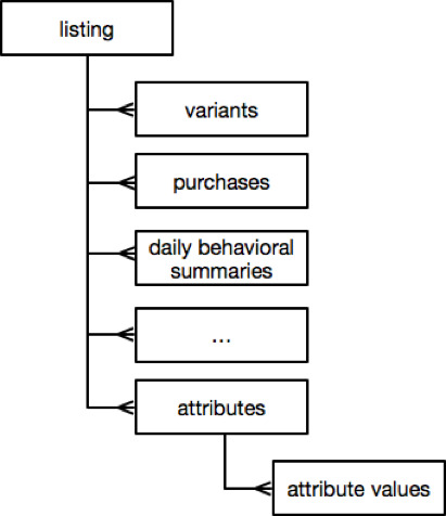
As mentioned above, listing data consists of many different kinds of records (entities), and resembles a hierarchical structure:

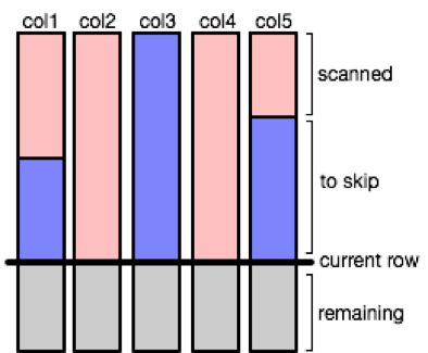
With data organized in columns, a mechanism is needed to align columns to the same logical record during scanning and also to recursively navigate columns in child records. To align columns at the same hierarchy level, we keep track of the currently scanned row position, and separately for the last accessed positions for all columns ever referenced by the query (query may access different columns on each row iteration). On each column access, we compare column position to the current row position, and skip over a range of column values (if necessary) to align that column to the current row. This alignment logic adds a few CPU cycles on each column access, and it results into a material overhead when scanning billions of values, but it simplifies the query API greatly.

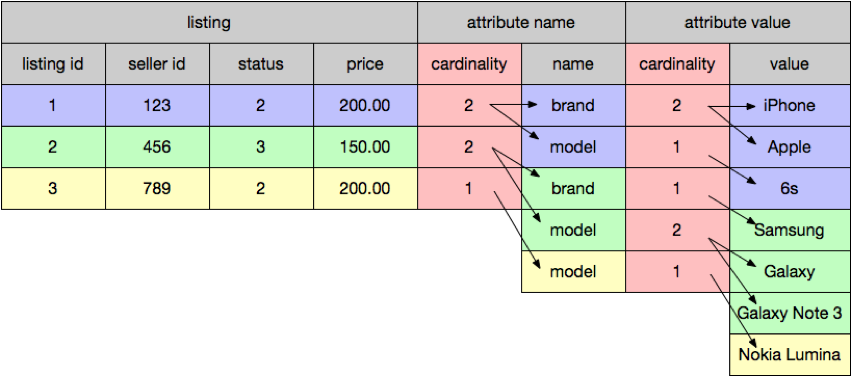
To align child entities, we introduce a special hidden “cardinality” column for each child containing the number of child records corresponding to the parent record. Incrementing the parent row position by 1 results in incrementing the child row position by the corresponding value contained in the cardinality column:

With the above table, we present a columnar dataset in the query API as an iterable collection of rows that is conceptually familiar to every developer (in pseudo-code):

for (listing <- listings)
  if (listing.sellerId == 123)
    for (attribute <- listing.attributes)
      for (value <- attribute.values)
        ...

The root (listing) iterator goes over all root records, and child iterators automatically terminate at the last child record for the currently iterated parent.

Data types

Analytics datasets contain mostly numeric data, or data that can be mapped to numeric types. In fact, most of the common types can be mapped to 32-bit integers:

• 64-bit integers (longs) map to two 32-bit integers for low and high bytes
• Booleans (flags) map to 0 or 1 (compression described below takes care of unused bits)
• Floating-point numbers can be represented as one or two 32-bit integers depending on the required precision
• Dates map to the number of days from an arbitrary “base” date (we’ve picked 1/1/2000).
• Time of day (with seconds precision) maps to the number of seconds from midnight
• Currency amounts map to integer amounts in the lowest denomination (for example, US dollar amounts are expressed in cents)

In cases when more than one 32-bit integer is needed for type mapping, we use multiple underlying integer columns to represent a single column in the dataset.

Type conversions are expensive when scanning billions of values, so it’s important that basic comparison operations can be performed on unconverted values (that is, the mappings are order-preserving).

We also use dictionaries for columns containing a relatively small number of distinct values, with each value converted to its index in the dictionary. Dictionaries work for any data type (for example, strings), including integers, in cases when a significant portion of distinct values are large by absolute value. Smaller numbers, like dictionary indexes, take less space when encoded/compressed. Dictionary indexes can be selected to preserve ordering, for example, lexicographic ordering for strings.

Another benefit of dictionaries is that the number of occurrences of each distinct value can be stored along with the value in page metadata. This helps with page pruning (for example, skipping pages not containing listings of a specific type) and allows the collection of statistics about encoded data without actually scanning it (for example, what’s the percentage of listings of a given type in a category).

We also support optional Bloom filters in metadata on columns that may be used for page pruning. For example, a Bloom filter on seller ID allows skipping pages that do not contain listings for specified sellers.

Columnar compression

For integer compression, we’ve developed a generic algorithm (IntRunLengthCodec) combining bit packing with Run-Length Encoding (RLE) and optional dictionary encoding. It detects whether RLE or bit packing is preferable for a block of numbers, and uses a heuristic on the percentage of distinct large values triggering use of dictionary. Apache Parquet uses a similar approach combining bit backing and RLE.

During decoding, IntRunLengthCodec supports skipping over ranges of values that is significantly faster than iteration, improving performance of column alignment.

For strings that do not fit into a dictionary, we use LZ4 compression in conjunction with IntRunLengthCodec to store string lengths. (We’ve started with Snappy, but LZ4 turned out a bit faster with similar compression ratios.) Both Snappy and LZ4 operate on blocks, allowing skipping over ranges of bytes for column alignment. Thus string columns are represented by two underlying columns, one with LZ4 compressed strings written back to back and another with the corresponding string lengths.

Compression ratios are highly dependent on the data being compressed. On average we achieve compression ratio of ~30 for the whole dataset, bringing the compressed size down to several terabytes.

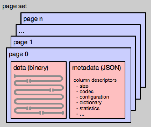
Page structure

We keep encoded column data separately from metadata that contains encoded column lengths and codec configurations. Metadata also contains dictionaries, serialized Bloom filters, and column statistics (min/max values, number of empty values, uncompressed data size, etc.)

On disk, column data for a page is written to a single binary file with columns written sequentially back to back. Metadata is written as a (compressed) JSON file. At run time, column data is memory mapped from the binary file, and metadata is loaded into an on-heap structure.

Pages belonging to the same subpartition are kept together as a “page set”. Page sets are dealt with atomically to ensure data consistency at subpartition level. When a newer version of subpartition page set is available, it’s loaded in memory, and the page set reference is swapped before unloading the older version.

At the time of page set loading, we also precompute frequently used aggregates (for example, daily GMV) and compact cross-references (for example, “relisting chains” where the same item was listed multiple times by a seller) across all pages. This data is stored on the heap together with the page set and can be used by queries.

We also provide an LRU cache at page set level for query results, so frequently executed queries can bypass page scanning on repeated executions with same parameters.

Schema API

Portico is implemented in Scala, and we leverage Scala DSL capabilities to provide friendly schema and query APIs.

The schema for a dataset is defined by extending the Schema class. (Code snippets are simplified, and class and method names are shortened for clarity):

class ListingSchema extends Schema("listings") {
  // columns
  val listingId = $long(key = true)
  val sellerId = $int(filtered = true)
  val status = $int()
  val price = $currency()
  ...

  // children
  val attributes = new AttributesSchema
  ...
}

class AttributeValuesSchema extends Schema {
  val value = $stringLz4(key = true)
}

class AttributesSchema extends Schema {
  val name = $stringDictionary(key = true)
  val values = new AttributeValuesSchema
}

The methods starting with '$' define columns along with configuration. (The '$' prefix was chosen to avoid name collisions in subclasses). In the above code, key = true designates a column as a part of the schema key. Key columns are used when merging incremental data into a page (see “Data ingestion” below). Specifying filtered = true enables Bloom filter creation. Column and child names are captured from Schema class field names via reflection. Column specifications are encapsulated in the ColumnSpecSet class and can be obtained from a schema instance.

At runtime, an instance of a ColumnSet representing a page (with references to memory-mapped column data and metadata) can be bound to an instance of Schema and scanned as follows:

val page: ColumnSet = ...
val listings: Schema = ...
val attributes: Schema = schema.attributes
val values: Schema = attributes.values
schema.bind(page)

while (listings.$hasMore) {
  listings.$advance()
  val listingId = listings.listingId.longValue
  val sellerId = listings.sellerId.intValue
  while (attributes.$hasMore) {
    attributes.$advance()
    val name = attributes.name.stringValue
    while (values.$hasMore) {
      values.$advance()
      val value = values.value.stringValue
      ...
    }
  }
}

Care is taken to ensure that column-access methods compile into Java primitives, so there is no primitive boxing and unboxing during scanning.

Column values can be converted into the target type during scanning. (Type annotation is added for clarity.)

val listingStartDate: LocalDate = listings.startDate.convertedValue

Column metadata is available directly from fields after binding, for example:

val sellerIdStats = listings.sellerId.stats

To support schema migration, binding resolves conflicts between columns and children in the schema and in the bound page:

• Columns are matched by name.
• Columns found in the page but missing in the schema are dropped.
• Columns found in the schema but missing in the page are substituted with columns containing type-specific empty values (0 for integers).
• If column type in the schema differs from column type in the page, automatic type conversion is applied (at scan time).
• Similarly, children are matched by name with non-matching children dropped or defaulted to all empty columns.

The above behavior can be overridden with an optional SchemaAdaptor passed into the bind() method. SchemaAdaptor allows custom type conversions, renaming columns and children, and also defaulting missing columns via a computation against other columns.

Adding data

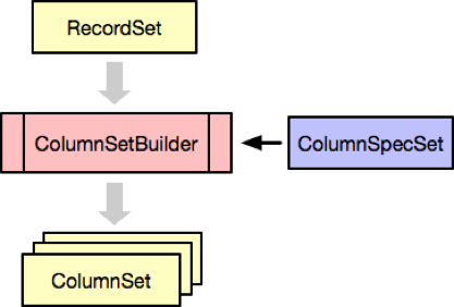
Schema iteration behavior over hierarchical records is defined in the RecordSet trait that Schema implements. RecordSet along with ColumnSpecSet (obtained from schema or created separately) serve as the input into ColumnSetBuilder, constructing a sequence of ColumnSets (pages) with fixed number of root records:

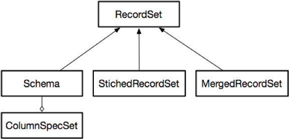
There are two other important implementations of RecordSet:

• StichedRecordSet takes a sequence of RecordSets and presents them as a single RecordSet.
• MergedRecordSet takes a RecordSet and a hierarchical collection of iterators over sorted incoming records (for example, parsed from CSV), and presents them as a single merged RecordSet. MergedRecordSet uses key fields to decide whether a record needs to be inserted or overwritten and to preserve the ordering of records throughout the hierarchy.

Thus, to add new data to a subpartition comprised of a sequence of pages (ColumnSets), we go through the following steps:

1. Bind existing pages to Schema (with optional SchemaAdaptor for schema migrations) to produce a sequence of RecordSets.
2. Construct a single StichedRecordSet from the above sequence of RecordSets.
3. Construct MergedRecordSet from StichedRecordSet with the incoming data.
4. Pass MergedRecordSet to ColumnSetBuilder to produce the resulting sequence of pages.

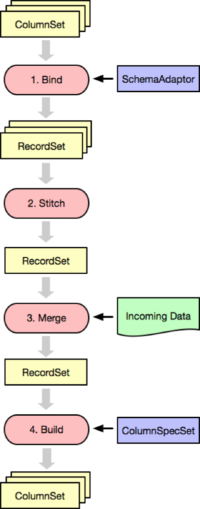
The above process relies on the fact that all records in the original ColumnSets and in the incoming data are sorted, and does not materialize intermediate RecordSets in memory (records are streamed), so it can be performed on inputs of arbitrary size.

Data distribution and coordination

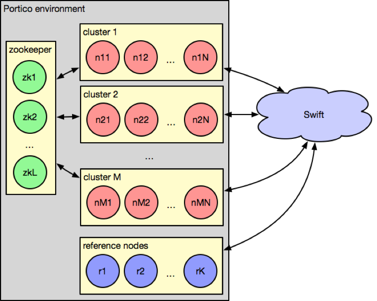
A Portico environment consists of one or more clusters. Each cluster contains all subpartitions comprising a dataset distributed across many nodes. Increasing the number of clusters increases redundancy and capacity (query throughput). The number of nodes within each cluster is determined by total heap and mapped memory needed to hold the dataset. Since memory-mapped files are paged from disk by the operating system, memory oversubscription is possible, however we try to keep oversubscription low to avoid excessive paging.

All nodes in an environment know about all other nodes in all clusters, so a single query can be distributed across the whole environment. We use Zookeeper for cluster membership, and consistent hashing (based on the Ketama algorithm) to minimize subpartition moves during rebalancing when nodes join or leave clusters. During rebalancing, nodes keep previously assigned subpartitions, so routing of queries to clusters that are being rebalanced is supported, improving environment availability and capacity.

Partitions that are frequently accessed due to seasonal or geographical access patterns can be dynamically configured with additional replicas to improve performance and availability.

With that, we achieve high availability and consistency of Portico environments, i.e. we guarantee that a successful query execution is performed exactly once against each requested partition/subpartition. Separation (by seller) and atomicity of subpartitions ensures that each listing is also evaluated exactly once.

In addition to cluster nodes, the Portico environment contains “reference” nodes that serve partition mappings used to limit the number of partitions where a query is dispatched (pruning); in our case, mapping from seller ID to all leaf categories where seller is present, as discussed in “Data organization.”

Portico environments run in eBay’s internal OpenStack cloud (Connected Commerce Cloud or C3), and datasets are persisted in OpenStack cloud storage (Swift).

Query execution

We leverage the map/reduce paradigm for query execution. Native Portico queries are written by extending the Query trait parameterized by query result type R:

trait Query[R] {
  def init(ctx: QueryContext, parameters: Option[JSON]): Unit
  def acceptPartitionKey(key: String ...): Boolean
  def execute(page: ColumnSet, key: String, ...): Option[R]
  def merge(result1: R, result2: R): R
  def onSubpartitionResult(result: R, key: String, ...): Option[R]
  def onPartitionResult(result: R, key: String, ...): Option[R]
  def onQueryResult(result: R, key): Option[R]
}

The init() method binds context and execution parameters to the query. Context provides access to the execution framework, and can be used to lookup locally provided services or to execute subqueries.

The execute() method scans a page and optionally produces a result. Query needs to define how results are combined in the merge() method. The execution framework invokes execute() method on each page for each partition or subpartition requested by the query. The merge() method is called recursively on the produced results, first with all results in a subpartition, then with all subpartition results in a partition, and finally with all partition results. The on...Result() callbacks can be optionally implemented by a query to apply special processing at these milestones during query execution.

We provide two specializations of the Query trait:

• SchemaQuery, where scanning occurs over a pre-bound schema
• SqlQuery, supporting ad-hoc SQL execution (using Apache Calcite)

During query execution, the framework collects statistics on how many values were scanned and skipped for each column in each subpartition. These statistics are sent back to the client along with the query result, and can be used for query tuning.

Clients submit queries to random nodes in a Portico environment over HTTP (all nodes are behind an HTTP load balancer). A named SchemaQuery can be submitted either as a precompiled JAR archive or as a Scala source text, in which case, Scala source is compiled into a JAR by the receiving node. JAR archives are distributed and stored on disk across clusters during execution, so subsequent query executions (with different parameters) don’t require JAR/source transfers. To isolate Portico clients, nodes use separate class loaders for each client, and same named query can be resubmitted/recompiled multiple times.

The receiving node computes distribution of subpartitions requested by the query across nodes in the environment and drops subpartitions (pruning by seller ID hash) that are not accepted by the query. If multiple nodes (in different clusters or replicas within cluster) contain the same requested subpartition, a heuristic is applied to balance the expected number of scanned records on each node and the distribution of requests across replicas. Query is then dispatched in parallel to selected nodes via HTTP API described above. Node-local query execution is also performed in parallel with multiple pages scanned concurrently, using all available CPUs. After all local results are merged into a single result, it’s serialized back to the calling node, and then, after merging all node results, back to the client.

Data ingestion

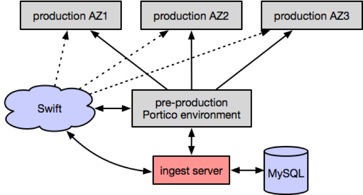
We merge new data into the Portico dataset daily. The new data is coming from Data Warehouse and data science feeds as separate flat CSV files for each entity comprising listing. There is a single “ingest” server responsible for feed preparation. Each feed is broken into fragments by leaf category ID and sorted by the corresponding key fields. Incoming feeds are tracked in a MySQL database, and fragments are stored in Swift. After all fragments are ready, the ingest server triggers the start of merge process in a Portico environment via HTTP API.

Nodes download incoming feed fragments from Swift for subpartitions they are responsible for and merge them into the corresponding page data, as described in “Adding data.” With multiple clusters, the node responsible for merging each subpartition is selected deterministically using hashes of cluster states and subpartition key.

Pages for merged subpartitions are uploaded to Swift, and updated across clusters in the environment via a node-to-node HTTP API with fallback to Swift. The ingest server monitors the overall progress of merging, and once merging is completed, it writes a build manifest to Swift, indicating a complete build. The ingest server also runs a report query to collect statistics (data sizes, record counts, etc.) for each partition in the new build, and persists this information in MySQL. This data is used to analyze sizing trends.

Portico environment can process queries during data ingestion, however the capacity during ingestion is degraded due to CPU time being spent on merging. We perform ingestion in a pre-production Portico environment and distribute new dataset builds into production environments in different availability zones (data centers) via the HTTP API, with fallback to Swift.

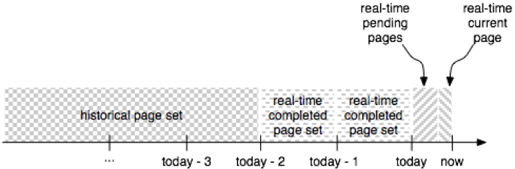
Near-real-time data

With several years of historical data, Portico supports a variety of analytics use cases, however, the historical data in Portico is at least one day old, as new data is merged daily. This gap is covered by near-real-time (NRT) data that is ingested from Kafka streams containing new and updated listings, purchases, small-window behavioral aggregates, etc. NRT data also temporarily covers historical data in case of delays in data warehouse extracts or historical data ingestion.

We chose to colocate NRT data for subpartitions with historical data on the same nodes. This helps in combining NRT and historical data for subpartitions in one pass in queries, reducing network trips and result sizes.

Like historical data, NRT data is broken into sequences of pages (page sets), however page size is determined by time window (for example, one hour) instead of the number of records. NRT page sets are grouped by day and dropped as new daily historical data arrives.

Unlike with historical data, we keep different entities separately with flat schemas, so scanning NRT data requires separate passes for each entity. Still, we guarantee that each record key occurs at most once within a page, and all records in a page are ordered. The deduplication and ordering happens in the “current” page that is kept on the heap and where the new data is being appended.

Seller Hub analytics performance

With Seller Hub expanding to the Big 4 markets, by November 2016, daily web traffic exceeded 4 million requests with an average of 400,000 unique visits. 99.47% of these requests achieve sub-second latency and all were ran on-the-fly on a dataset size of over 100 TB, compressed to a size of 3.6 TB and memory-mapped. With over three years of behavioral impression data and over four years of listing data, eBay’s sellers for the first time are able to perform real time analytics on their listing impressions, sales conversion rate, price trends, and those of their competitors.

To achieve this performance, Seller Hub’s queries are optimized to take advantage of several features that were designed for best performance and optimum capacity utilization.

As described in “Data organization,” most of our sellers tend to focus their businesses on a small subset of trending categories such as Fashion, Electronics, and DVDs, and trending categories tend to change with seasonality. These large leaf categories are sub-partitioned by seller ID hash and have most of their traffic balanced across the clusters. Also, from analyzing the access pattern of Seller Hub’s sellers and their geographic time zones, Portico is able to dynamically configure additional replica sets for these trending categories to further increase query performance.

For seller-centric queries, queries make extensive use of Bloom filters and column statistics described in “Page Structure” to prune pages that do not contain listings in the specified date ranges for that seller. For category-level aggregation queries, such as finding last 30- and 365-days markets’ GMV, these results are pre-computed once during the loading of sub-partitions and cached for the day until the next daily build, as described in “Data ingestion.” Lastly, over 80% of the queries are sent using default 30-day time window, caching the query result of this frequently accessed date range in the query cache, once computed, greatly improved the average performance.

Next steps

• The Portico team is still working on exposing NRT data in Seller Hub.
• We would like to improve Calcite integration, primarily around projection and filter optimizations.
• We are following the Apache Arrow project and considering it as a potential foundation for native replacement of codecs and schema API.

---

Powered by QuickLaTeX.