Peer Groups in Empirical Bayes

In a post from February, I sang the praises of Empirical Bayes, and showed how eBay uses it to judge the popularity of an item. This post discusses an important practical issue in using Empirical Bayes which I call “Peer Groups”.

(Update, August 29, 2017: I just discovered that the book, Computer Age Statistical Inference by Efron & Hastie, also discusses peer groups in section 15.6, although they call it “relevance” rather than “peer groups.”)

First, a quick summary of the February post. The popularity of an item with multiple copies available for sale can be measured by the number sold divided by the number of times the item has been viewed, sales/impressions for short. The problem was how to interpret the ratio sales/impressions when the number of impressions is small and there might not be any sales yet. The solution was to think of the ratio as a proxy for the probability of sale (call it $\pi$ ), and use Bayes theorem to estimate $\pi$ . Bayes theorem requires a prior probability, which I estimated using some of eBay’s voluminous sales data. This method is called Empirical Bayes because the prior is determined empirically, using the data itself.

That brings me to peer groups. When computing the prior probability that an item gets a sale, I want to base it on sales/impressions data from similar items, which I call a peer group. For example if the item is a piece of jewelry, the peer group might be all items of jewelry listed on eBay in the past month. I can get more specific. If the item is new, then the peer group might be restricted to new items. If the list price is $138, the peer group might be further restricted to items whose price was between $130 and $140, and so on.

Once you have identified a peer group and used it to estimate the prior probability, you use Bayes theorem to combine that with the observed count of sales and impressions to compute the probability of sale. This is the number you want—the probability that the next impression will result in a sale. It is called the posterior probability, to distinguish it from the prior probability.

There’s a tension in selecting the peer group. You might think that a peer group more strongly constrained to be similar to the item under consideration will result in a better prior and therefore a better estimate of the probability of a sale. But as the peer group gets smaller and smaller, the estimate of the prior based on the group becomes noisier and less reliable.

Which finally brings me to the subject of this post. In the case where the peer group is specified by a continuous variable like price, you can get the best of both worlds—a narrowly defined peer group and a lot of data (hence low noise) to estimate the prior parameters.

The idea

The idea is modeling. If the prior depends on the price , and if there is a model for the dependence, the same data used to compute the prior can be used to find the model. Then an item of price is assigned the prior given by the model at , which is essentially the peer group of all items with exactly price . Since this prior is a prediction of the model, it indirectly uses all the data, since the model depends on the entire data set.

Dependence on price

What is needed to apply Bayes theorem is not a single probability $\pi$ , but rather a probability distribution on $\pi$ . I assume the distribution of $\pi$ is a Beta distribution $B(\alpha, \beta)$ , which has two parameters. Specifying the prior means providing values of $\alpha$ and $\beta$ .

So our idea is to see if there is a simple parametrized function that explains the dependence of $\alpha(p)$ and $\beta(p)$ on the price . The beta distribution $B(\alpha, \beta)$ has a mean of $\mu = \alpha/(\alpha + \beta)$ . As a first step, I examine the dependence of $\mu$ (rather than $\alpha$ and $\beta$ ) on price.

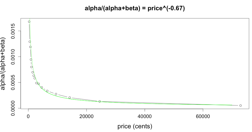
The fit to the power law $\mu \propto \beta^{-0.67}$ is very good. The values of $\alpha$ and $\beta$ are noisier than $\mu$ . But I do know one thing: sales/impressions is small, so that $\mu$ is small, and therefore $\alpha \ll \beta$ so $\mu \approx \alpha/\beta$ . It follows that if $\alpha$ and $\beta$ fit a power law, so would $\mu$ . Thus a power law for $\alpha$ and $\beta$ is consistent with the plot above.

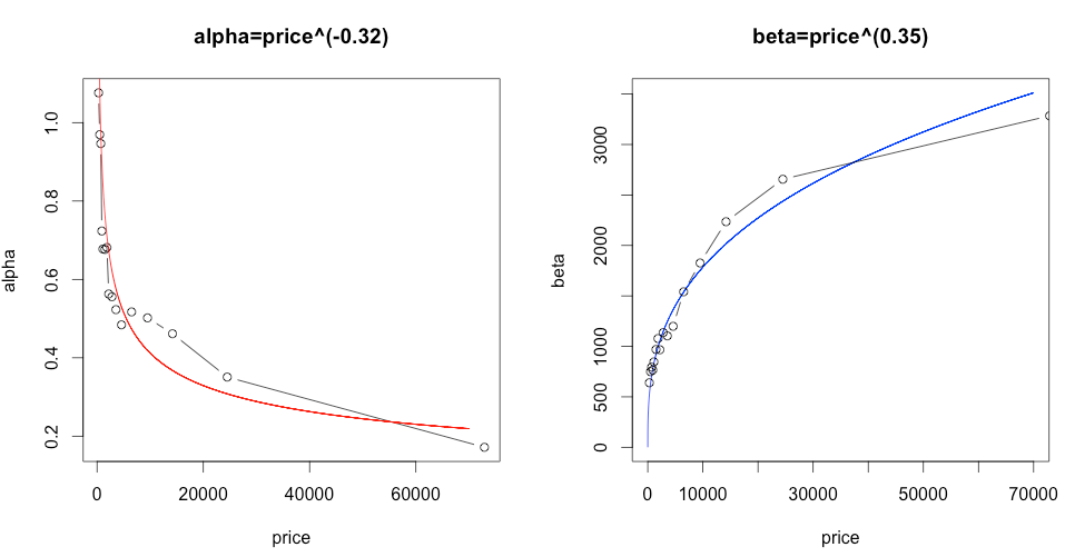
Here are plots of $\alpha(p)$ and $\beta(p)$ . Although somewhat noisy, their fits to power laws are reasonable. And the exponents add as expected: the exponent for $\alpha$ is , for $\beta$ is 0.35, and for $\mu = \alpha/(\alpha + \beta) \approx \alpha/\beta$ is .

Details

Once the form of the dependence of $\alpha$ and $\beta$ on price is known, the Empirical Bayes computations proceed as usual. Instead of having to determine two constants $\alpha$ and $\beta$ , I use Empirical Bayes to determine four constants , , , and , where

$\alpha(p) = c_1 p^{c_2} \qquad \beta(p) = c_3 p^{c_4}$

The details are in the February posting, so I just summarize them here. The are computed using maximum likelihood as follows. The probability of seeing a sales/impressions ratio of is

$q_i(\alpha, \beta) = \binom{n_i}{k_i} \frac{B(\alpha + k_i, n_i + \beta - k_i)}{B(\alpha, \beta)}$

and max likelihood maximizes the product $\prod_i q_i(\alpha, \beta)$ or equivalently the log

$l(\alpha, \beta) = \sum_i \log q_i(\alpha, \beta)$

Instead of maximizing a function of two variables $\alpha$ , $\beta$ maximize

$l(c_1, c_2, c_3, c_4) = \sum_i \log q_i(c_1 p_i^{c_2}, c_3 p_i^{c_4})$

Once you have computed , then an item with sales out of impressions at price has a posterior probability of $(\alpha + k)/(\alpha + \beta + n) =(c_1 p^{c_2} + k)/(c_1 p^{c_2} + c_3 p^{c_4} + n)$ .

Beta regression

When people hear about the peer group problem with a beta distribution prior, they sometimes suggest using beta regression. This suggestion turns out not to be as promising as it first seems. In this section I will dig into beta regression, but it is somewhat of a detour so feel free to skip over it.

When we first learn about linear regression, we think of points on the plane and drawing the line that best fits them. For example the -coordinate might be a person’s height, the coordinate is the person’s weight, and the line shows how (on the average) weight varies with height.

A more sophisticated way to think about linear regression is that each point represents a random variable . In the example above, is a height, and represents the distribution of weights for people of height . The height of the line at represents the mean of . If the line is , then has a normal distribution with mean .

Beta regression is a variation when has a beta distribution instead of a normal distribution. If the satisfy $0 \leq y_i \leq 1$ they are clearly not from a normal distribution, but might be from a beta distribution. In beta regression you assume that is distributed like $B(\alpha_i, \beta_i)$ where the mean $\mu_i = \alpha_i/(\alpha_i + \beta_i)$ is , or perhaps a function of . The theory of beta regression tells you how to take a set of and compute the coefficients and .

But in our situation we are not given from a beta distribution. The beta distribution is the unknown (latent) prior distribution. So it’s not obvious how to apply beta regression to get $\alpha(p)$ and $\beta(p)$ .

Summary

Empirical Bayes is a technique that can work well for problems with large amounts of data. It uses a Bayesian approach that combines a prior and a particular item’s data to get a posterior probability for that item. For us the data is sales/impressions for the item, and the posterior is the probability that an impression for that item results in a sale.

The prior is based on a set of parameters, which for a beta distribution is $\{\alpha, \beta\}$ . The parameters are chosen to make the best possible fit of the posterior to a subset of the data. But what subset?

There’s a tradeoff. If the subset is too large, it won’t be representative of the item under study. If it is too small, the estimates of the parameters will be very noisy.

If the subset is parametrized by a continuous variable (price in our example), you don’t need to decide how to make the tradeoff. You use the entire data set to build a model of how the parameters vary with the variable. And then when computing the posterior of an item, you use the parameters given by the model. In our example, I use the data to compute constants $c_1, \ldots c_4$ . If the item has price , sales and impressions, then the parameters of the prior are $\alpha = c_1p^{c_2}$ and $\beta = c_3p^{c_4}$ and the estimated probablity of a sale (the posterior) is $(c_1 p^{c_2} + k)/(c_1 p^{c_2} + c_3 p^{c_4} + n)$ .

Tags: Applied Math, Search Science